Function Reference: gustafson_kessel
- Function File: cluster_centers = gustafson_kessel (input_data, num_clusters)
- Function File: cluster_centers = gustafson_kessel (input_data, num_clusters, cluster_volume)
- Function File: cluster_centers = gustafson_kessel (input_data, num_clusters, cluster_volume, options)
- Function File: cluster_centers = gustafson_kessel (input_data, num_clusters, cluster_volume, [m, max_iterations, epsilon, display_intermediate_results])
- Function File: [cluster_centers, soft_partition, obj_fcn_history] = gustafson_kessel (input_data, num_clusters)
- Function File: [cluster_centers, soft_partition, obj_fcn_history] = gustafson_kessel (input_data, num_clusters, cluster_volume)
- Function File: [cluster_centers, soft_partition, obj_fcn_history] = gustafson_kessel (input_data, num_clusters, cluster_volume, options)
- Function File: [cluster_centers, soft_partition, obj_fcn_history] = gustafson_kessel (input_data, num_clusters, cluster_volume, [m, max_iterations, epsilon, display_intermediate_results])
Using the Gustafson-Kessel algorithm, calculate and return the soft partition of a set of unlabeled data points.
Also, if display_intermediate_results is true, display intermediate results after each iteration. Note that because the initial cluster prototypes are randomly selected locations in the ranges determined by the input data, the results of this function are nondeterministic.
The required arguments to gustafson_kessel are:
- input_data: a matrix of input data points; each row corresponds to one point
- num_clusters: the number of clusters to form
The third (optional) argument to gustafson_kessel is a vector of cluster volumes. If omitted, a vector of 1’s will be used as the default.
The fourth (optional) argument to gustafson_kessel is a vector consisting of:
- m: the parameter (exponent) in the objective function; default = 2.0
- max_iterations: the maximum number of iterations before stopping; default = 100
- epsilon: the stopping criteria; default = 1e-5
- display_intermediate_results: if 1, display results after each iteration, and if 0, do not; default = 1
The default values are used if any of the four elements of the vector are missing or evaluate to NaN.
The return values are:
- cluster_centers: a matrix of the cluster centers; each row corresponds to one point
- soft_partition: a constrained soft partition matrix
- obj_fcn_history: the values of the objective function after each iteration
Three important matrices used in the calculation are X (the input points to be clustered), V (the cluster centers), and Mu (the membership of each data point in each cluster). Each row of X and V denotes a single point, and Mu(i, j) denotes the membership degree of input point X(j, :) in the cluster having center V(i, :).
X is identical to the required argument input_data; V is identical to the output cluster_centers; and Mu is identical to the output soft_partition.
If n denotes the number of input points and k denotes the number of clusters to be formed, then X, V, and Mu have the dimensions:
                                     1    2   ...  #features
                               1 [[                           ]
    X  =  input_data       =   2  [                           ]
                              ... [                           ]
                               n  [                           ]]

                                     1    2   ...  #features
                               1 [[                           ]
    V  =  cluster_centers  =   2  [                           ]
                              ... [                           ]
                               k  [                           ]]

                                     1    2   ...   n
                               1 [[                    ]
    Mu  =  soft_partition  =   2  [                    ]
                              ... [                    ]
                               k  [                    ]]
See also: fcm, partition_coeff, partition_entropy, xie_beni_index
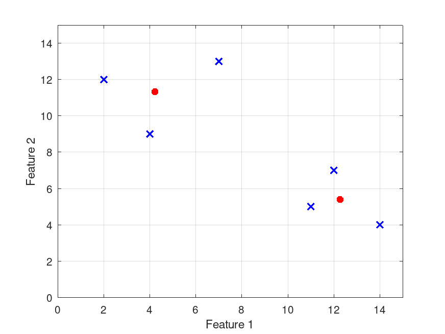
Example: 1
 ## This demo:
 ##    - classifies a small set of unlabeled data points using
 ##      the Gustafson-Kessel algorithm into two fuzzy clusters
 ##    - plots the input points together with the cluster centers
 ##    - evaluates the quality of the resulting clusters using
 ##      three validity measures: the partition coefficient, the
 ##      partition entropy, and the Xie-Beni validity index
 ##
 ## Note: The input_data is taken from Chapter 13, Example 17 in
 ##       Fuzzy Logic: Intelligence, Control and Information, by
 ##       J. Yen and R. Langari, Prentice Hall, 1999, page 381
 ##       (International Edition).

 ## Use gustafson_kessel to classify the input_data.
 input_data = [2 12; 4 9; 7 13; 11 5; 12 7; 14 4];
 number_of_clusters = 2;
 [cluster_centers, soft_partition, obj_fcn_history] = ...
   gustafson_kessel (input_data, number_of_clusters)

 ## Plot the data points as small blue x's.
 figure ('NumberTitle', 'off', 'Name', 'Gustafson-Kessel Demo 1');
 for i = 1 : rows (input_data)
   plot (input_data(i, 1), input_data(i, 2), 'LineWidth', 2, ...
         'marker', 'x', 'color', 'b');
   hold on;
 endfor

 ## Plot the cluster centers as larger red *'s.
 for i = 1 : number_of_clusters
   plot (cluster_centers(i, 1), cluster_centers(i, 2), ...
         'LineWidth', 4, 'marker', '*', 'color', 'r');
   hold on;
 endfor

 ## Make the figure look a little better:
 ##    - scale and label the axes
 ##    - show gridlines
 xlim ([0 15]);
 ylim ([0 15]);
 xlabel ('Feature 1');
 ylabel ('Feature 2');
 grid
 hold

 ## Calculate and print the three validity measures.
 printf ("Partition Coefficient: %f\n", ...
         partition_coeff (soft_partition));
 printf ("Partition Entropy (with a = 2): %f\n", ...
         partition_entropy (soft_partition, 2));
 printf ("Xie-Beni Index: %f\n\n", ...
         xie_beni_index (input_data, cluster_centers, ...
         soft_partition));

Iteration count = 1,  Objective fcn = 45.858745
Iteration count = 2,  Objective fcn = 32.524816
Iteration count = 3,  Objective fcn = 26.049556
Iteration count = 4,  Objective fcn = 25.673979
Iteration count = 5,  Objective fcn = 25.652426
Iteration count = 6,  Objective fcn = 25.647293
Iteration count = 7,  Objective fcn = 25.645559
Iteration count = 8,  Objective fcn = 25.644959
Iteration count = 9,  Objective fcn = 25.644752
Iteration count = 10,  Objective fcn = 25.644681
Iteration count = 11,  Objective fcn = 25.644657
Iteration count = 12,  Objective fcn = 25.644648
Iteration count = 13,  Objective fcn = 25.644645
Iteration count = 14,  Objective fcn = 25.644644
Iteration count = 15,  Objective fcn = 25.644644
Iteration count = 16,  Objective fcn = 25.644644
Iteration count = 17,  Objective fcn = 25.644644
Iteration count = 18,  Objective fcn = 25.644644
Iteration count = 19,  Objective fcn = 25.644644
Iteration count = 20,  Objective fcn = 25.644644
Iteration count = 21,  Objective fcn = 25.644644
cluster_centers =

   12.2661    5.3877
    4.2228   11.3276

soft_partition =

   0.065974   0.109473   0.129499   0.976470   0.971912   0.987408
   0.934026   0.890527   0.870501   0.023530   0.028088   0.012592

obj_fcn_history =

 Columns 1 through 10:

   45.859   32.525   26.050   25.674   25.652   25.647   25.646   25.645   25.645   25.645

 Columns 11 through 20:

   25.645   25.645   25.645   25.645   25.645   25.645   25.645   25.645   25.645   25.645

 Column 21:

   25.645

Partition Coefficient: 0.888484
Partition Entropy (with a = 2): 0.308027
Xie-Beni Index: 0.107028
|
Example: 2
## This demo:
## - classifies three-dimensional unlabeled data points using
## the Gustafson-Kessel algorithm into three fuzzy clusters
## - plots the input points together with the cluster centers
## - evaluates the quality of the resulting clusters using
## three validity measures: the partition coefficient, the
## partition entropy, and the Xie-Beni validity index
##
## Note: The input_data was selected to form three areas of
## different shapes.
## Use gustafson_kessel to classify the input_data.
input_data = [1 11 5; 1 12 6; 1 13 5; 2 11 7; 2 12 6; 2 13 7;
3 11 6; 3 12 5; 3 13 7; 1 1 10; 1 3 9; 2 2 11;
3 1 9; 3 3 10; 3 5 11; 4 4 9; 4 6 8; 5 5 8; 5 7 9;
6 6 10; 9 10 12; 9 12 13; 9 13 14; 10 9 13; 10 13 12;
11 10 14; 11 12 13; 12 6 12; 12 7 15; 12 9 15;
14 6 14; 14 8 13];
number_of_clusters = 3;
[cluster_centers, soft_partition, obj_fcn_history] = ...
gustafson_kessel (input_data, number_of_clusters, [1 1 1], ...
[NaN NaN NaN 0])
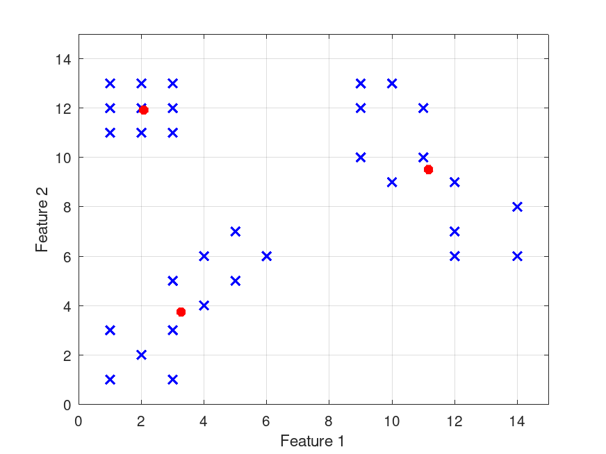
## Plot the data points in two dimensions (using features 1 & 2)
## as small blue x's.
figure ('NumberTitle', 'off', 'Name', 'Gustafson-Kessel Demo 2');
for i = 1 : rows (input_data)
plot (input_data(i, 1), input_data(i, 2), 'LineWidth', 2, ...
'marker', 'x', 'color', 'b');
hold on;
endfor
## Plot the cluster centers in two dimensions
## (using features 1 & 2) as larger red *'s.
for i = 1 : number_of_clusters
plot (cluster_centers(i, 1), cluster_centers(i, 2), ...
'LineWidth', 4, 'marker', '*', 'color', 'r');
hold on;
endfor
## Make the figure look a little better:
## - scale and label the axes
## - show gridlines
xlim ([0 15]);
ylim ([0 15]);
xlabel ('Feature 1');
ylabel ('Feature 2');
grid
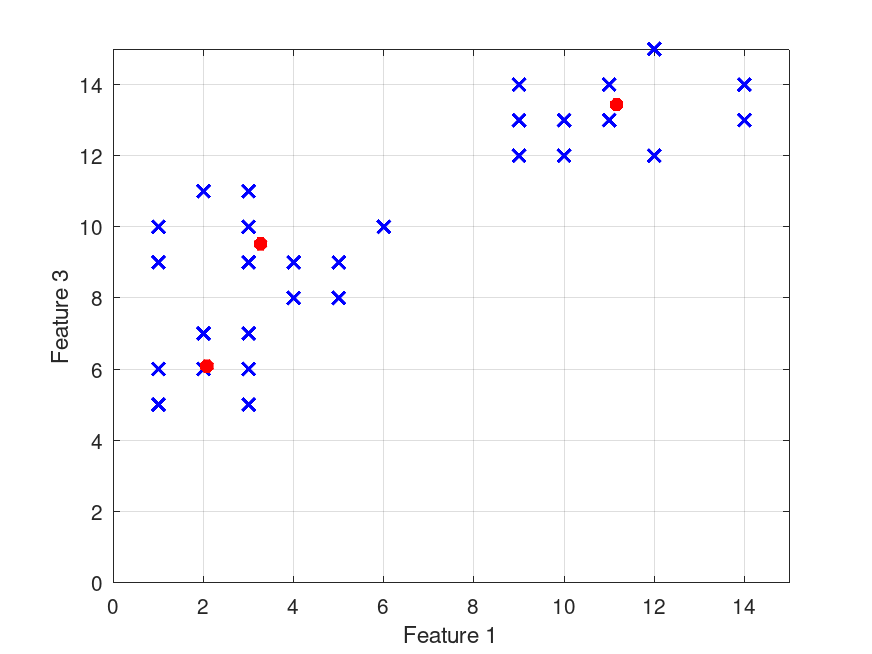
## Plot the data points in two dimensions
## (using features 1 & 3) as small blue x's.
figure ('NumberTitle', 'off', 'Name', 'Gustafson-Kessel Demo 2');
for i = 1 : rows (input_data)
plot (input_data(i, 1), input_data(i, 3), 'LineWidth', 2, ...
'marker', 'x', 'color', 'b');
hold on;
endfor
## Plot the cluster centers in two dimensions
## (using features 1 & 3) as larger red *'s.
for i = 1 : number_of_clusters
plot (cluster_centers(i, 1), cluster_centers(i, 3), ...
'LineWidth', 4, 'marker', '*', 'color', 'r');
hold on;
endfor
## Make the figure look a little better:
## - scale and label the axes
## - show gridlines
xlim ([0 15]);
ylim ([0 15]);
xlabel ('Feature 1');
ylabel ('Feature 3');
grid
hold
## Calculate and print the three validity measures.
printf ("Partition Coefficient: %f\n", ...
partition_coeff (soft_partition));
printf ("Partition Entropy (with a = 2): %f\n", ...
partition_entropy (soft_partition, 2));
printf ("Xie-Beni Index: %f\n\n", ...
xie_beni_index (input_data, cluster_centers, ...
soft_partition));
cluster_centers =
3.2679 3.7416 9.5189
11.1675 9.5123 13.4360
2.0744 11.9210 6.0810
soft_partition =
Columns 1 through 7:
1.9129e-02 9.7022e-03 1.0643e-02 2.4975e-02 8.9273e-05 1.9737e-02 2.1778e-02
1.1157e-02 7.1681e-03 9.2569e-03 1.3793e-02 6.1636e-05 1.8522e-02 1.0694e-02
9.6971e-01 9.8313e-01 9.8010e-01 9.6123e-01 9.9985e-01 9.6174e-01 9.6753e-01
Columns 8 through 14:
4.1337e-02 2.3680e-02 9.6778e-01 9.1988e-01 9.5714e-01 9.2049e-01 9.9099e-01
2.5264e-02 2.0998e-02 9.2635e-03 1.8979e-02 1.3117e-02 2.2734e-02 2.4882e-03
9.3340e-01 9.5532e-01 2.2954e-02 6.1140e-02 2.9744e-02 5.6773e-02 6.5221e-03
Columns 15 through 21:
8.8919e-01 9.8157e-01 8.2057e-01 8.7617e-01 8.2343e-01 8.1787e-01 1.3809e-01
3.1044e-02 4.4868e-03 2.9448e-02 2.6948e-02 3.3445e-02 5.4462e-02 7.2960e-01
7.9764e-02 1.3944e-02 1.4998e-01 9.6877e-02 1.4313e-01 1.2767e-01 1.3231e-01
Columns 22 through 28:
4.4812e-02 5.9662e-02 4.7384e-02 1.0958e-01 8.6143e-03 5.4236e-02 8.1535e-02
9.0208e-01 8.6338e-01 9.0000e-01 7.8177e-01 9.8041e-01 8.8735e-01 8.1781e-01
5.3109e-02 7.6958e-02 5.2618e-02 1.0865e-01 1.0973e-02 5.8411e-02 1.0065e-01
Columns 29 through 32:
4.1312e-02 3.1916e-02 2.5981e-02 5.2999e-02
8.9517e-01 9.2117e-01 9.3144e-01 8.7447e-01
6.3519e-02 4.6918e-02 4.2584e-02 7.2535e-02
obj_fcn_history =
Columns 1 through 10:
225.36 174.39 162.04 153.98 148.21 143.92 140.45 137.19 133.86 130.30
Columns 11 through 20:
126.69 123.61 121.64 120.69 120.29 120.13 120.07 120.05 120.04 120.03
Columns 21 through 30:
120.03 120.03 120.03 120.03 120.03 120.03 120.03 120.03 120.03 120.03
Columns 31 through 33:
120.03 120.03 120.03
Partition Coefficient: 0.841843
Partition Entropy (with a = 2): 0.472419
Xie-Beni Index: 0.192632
|